Accelerating the Super-Resolution NIR-SPI system using CNN

Single image super-resolution (SR) methods aim at recovering high-resolution (HR) images from given low-resolution (LR) ones. SR Algorithms are mostly learning-based methods that learn a mapping between the LR and HR image spaces (see Fig.1) . Among SR methods present in the literature, there are Super-Resolution Convolutional Neural Networks and Fast Super-Resolution Convolutional Neural Networks, among the most used ones.

Fig.1. Comparative performance of the SRCNN and FSRCNN super-resolution method.

FSRCNN: A improvement of the SRCNN method, which adopts the original low-resolution image as input. This method is divided into five parts:

• Feature Extraction: Bicubic interpolation in previous SRCNN is replaced by 5×5 conv.

• Shrinking: 1×1 conv is done to reduce the number of feature maps from d to s where s<<d.

• Non-Linear Mapping: Multiple 3×3 layers are to replace a single wide one

• Expanding: 1×1 conv is done to increase the number of feature maps from s to d

• Deconvolution: 9×9 filters are used to reconstruct the HR image.

The FSRCNN is different from SRCNN mainly in three aspects. First, FSRCNN adopts the original low-resolution image as input without bicubic interpolation. A deconvolution layer is introduced at the end of the network to perform upsampling. Second, the non-linear mapping step in SRCNN is replaced by three steps in FSRCNN: the shrinking, the mapping, and the expanding step. Third, FSRCNN adopts smaller filter sizes and a deeper network structure. These improvements provide FSRCNN with better performance but lower computational cost than SRCNN.

Fig.2. Network structures of the SRCNN and FSRCNN methods.

Structure of FSRCNN

For the implementation of the FSRCNN, we implemented a model with eight layers, where layer 1 is the Feature extraction, layer 2 is, layers 3–6 are denoted to figure 3, layer seven carrier out expanding, and layer 8 performs the deconvolution function. The layers are defined as follows:

• Conv. Layer 1 "Feature extraction": 56 filters of size 1 x 5 x 5.Activation function: PReLU. Output: 56 feature maps; parameters: 1 x 5 x 5 x 56 = 1400 weights and 56 biases

• Conv. Layer 2 "Shrinking": 12 filters of size 56 x 1 x 1. Activation function: PReLU. Output: 12 feature maps; parameters: 56 x 1 x 1 x 12 = 672 weights and 12 biases

• Conv. Layers 3–6 "Mapping": 4 x 12 filters of size 12 x 3 x 3. Activation function: PReLU. Output: HR feature maps; parameters: 4 x 12 x 3 x 3 x 12 = 5184 weights and 48 biases

• Conv. Layer 7 "Expanding": 56 filters of size 12 x 1 x 1. Activation function: PReLU.Output: 12 feature maps; parameters: 12 x 1 x 1 x 56 = 672 weights and 56 biases

• DeConv Layer 8 "Deconvolution": One filter of size 56 x 9 x 9. Activation function: PReLU. Output: 12 feature maps; parameters: 56 x 9 x 9 x 1 = 4536 weights and 1 bias

Fig.3.Structure of FSRCNN.

Fig.4: SPI 2D image reconstruction using Batch-OMP algorithm in combination with FSRCNN for the scanning methods: Basic, Hilbert, Zig-Zag, and Spiral. As the test object, a Sphere with 50 mm of diameter placed at 25 cm focal length:(a-d)SPI reconstruction of the 8x8 image using the following scanning methods Basic, Hilbert, Zig-Zag, and Spiral respectively, (e-h) post-processing a method based on the application of a bilateral filter, and(i-l)SPI image obtained after applying the FSRCNN approach.

2D/3D image reconstruction algorithms on GPU

Single image processing time is critical for generating 2D digital images and video streams in SPI for real-time applications. To reduce the time required by the 2D image processing system, to generate an image, we determined the minimum number of illumination patterns equivalent to a compression factor of 2% to be able to adapt the OMP-Batch Algorithm [68] based on hardware architecture and a GPU. The OMP-Batch Algorithm [68], compared with other compressed sensings (CS) Algorithms such as OMP and OMP-Cholesky, presents improvements in processing time because they do not make operations of the inverse matrix. On the contrary, using the definition of the Gram-matrix, G=ATA, initially, pre-calculating Gram-matrix G with initial projection i, where an initial projection as p0=ATy is defined. This allows finding the new atom Ai, which will be used as stop criteria for the system solution calculation. For implementing the OMP-Batch algorithm, we defined four kernels that must operate in parallel.

• The input information is defined in the first kernel, the Gram-matrix (G= ATA) is generated, and the residual norm r is calculated.

• The second kernel was used to calculate the new atom Ai.

• The third kernel was used to calculate the Cholesky decomposition, where the matrix N×N was defined to calculate the matrix L using.

• The fourth kernel was used to calculate the matrix space-vector product and the normal error e.

Implementation of the OMP-Batch algorithm on GPU

For the implementation of the OMP-Batch algorithm on GPU, we must take into consideration some details, such as: The Cholesky factorization scheme, the memory layout, the matrix batched-matrix products, normalized columns of the dictionary, packed representation (library Python), and efficient batched argmax

Memory layout: The main bottleneck in the process is matrix multiplication. To get more speed, transpose the matrix columns, as one column can span into a single line in the memory. After that, we apply the operation of matrix multiplication.

Cholesky factorization scheme: The OMP-Batch uses an inverse Cholesky factorization method based on the precomputedATy, and ATA, in the parallel computing environment. We seek to calculate Lk, which we do not need to store in each iteration. We only need to perform are iteration

to obtain the new projections w.

Matrix batched-matrix products: A less-known fact is that we can sometimes get higher performance. If we apply the matrix times batched-matrix product. We can see that this matrix times batched-

vector product is equivalent to a simple matrix-matrix product, with which we can use the library BLAS (Basic Linear Algebra Subprograms) most efficiently.

Normalized columns of the used dictionary: The main approach to speeding up the algorithm is to minimize the number of operations to perform each iteration. Many algorithms assume normalized columns in A such that correlation projection⟨an, rk−1⟩/∥an∥ turns into a simple projection ⟨an, rk−1⟩=[ATrk−1]. This is valid since the algorithm is invariant to the column norm, as it will be divided out in the correlation step, and lastly, the least-squares estimateˆyk=AAT y=A,argminx∈Rk∥y−Ax∥ is unique. Thus, it is also invariant to column scaling. For the final estimate ˆx from ATAˆx=ATy, one should not use the pre-normalized A, or at least the scale ˆxappropriately (by the reciprocal of the column norm) to account for this.

Packed representation: Specialized calls for batched matrix-matrix multiplication, batched Cholesky factorization and batched triangular system solving for GPU exist. In our approach, we use the PyTorch library.

Efficient batched argmax: A core part of the OMP loop is argmax, which can be performed on a batch by k= arg maxK|p|. One issue is that abs (|p|) creates an intermediate M×N array in the first pass, and then a second pass over this is needed to get the ”argmax.” The ”argmax” line takes 5-25% of the

GPU computation time. To optimize this, we applied libraries of CuPy to increase the speed-up of computation. The function arg maxK is compiled in C++ and called in Python as an external function.

By implementing the OMP-Batch on GPU, we can reach an acceleration of x27 compared to running the same algorithm on the CPU (see Fig. 1). In table 1, we compared the complexity and memory requirements of the different OMP reconstruction test algorithms.

Table 1. Comparison of complexities and memory requirements in the k-th iteration,

where the dictionary Φ is MxN.

Fig.1.Comparative reconstruction time for running the OMP-Batch algorithm on different platforms: CPU Intel i5 OMP Basic, CPU-1 with Linux OMP basic, GPU-VO using Pytourch GPU reach an acceleration x 17 on Jetson Nano, GPU-V1 using PyTorch GPU compile in C++ the function arg maxK with an acceleration x 27 on Jetson Nano

---

Toward a single-pixel near-infrared low-resolution 2D image reconstruction strategy using GPU

In this article, we propose a method to be used for the reconstruction of single-pixel near-infrared (SPI-NIR) low-resolution 2D images using active illumination with a peak wavelength of 1550 nm that is based on Batch Orthogonal Matching (Batch-OMP) processing algorithms and a region definition in

the projection sequence of Hadamard illumination patterns using the genetic algorithm(GA). Different methods to generate Hadamard pattern sequences have been reported, mostly based on switching the illumination sequence on and off to improve the reconstructed image quality, thereby increasing the Structural Similarity Index Measure (SSIM) level and reducing the processing time. These methods are efficient for image sizes of>64x64virtual pixels, but for lower resolutions with small coherence areas Ach, the SNR level of the reconstructed image is very low, which makes other methods, such as those using the Zig-Zag or Hilbert filling curves for the scanning path, an option for the reconstruction of SPI-NIR low-resolution images. Because in the present application, we deal with low-resolution (size image 8 x 8 virtual pixels) SPI-NIR images, we present a solution to improve the obtained image quality (aiming at PSNR>10dBand SSIM>0.5) that is based on the use of a specific scanning path and a combination of a genetic algorithm to define the switching sequences of the Hadamard patterns, using Batch-OMP algorithm for image reconstruction in the processing time range between 20 and 35 ms.

Fig.1. Schematic diagram of Hadamard pattern generation using GA: (a) population with Hadamard parent patterns is generated to illuminate the object, (b) after the cost function measurement, these patterns are ranked using the matrix Hp, (c) each new pattern is created through changes in patterns using a mutation operation of the values, (d) the mutated offspring patterns replace the parent generation patterns. These steps are repeated in every generation.

Hadamard genetic algorithm (GA) for region-projection

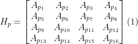
To define the projection areas Ap, we start by dividing all the Hadamard N x N projection patterns required (for our application, the maximum required number of patterns is 64) into groups of N / 4, each containing a number of N / 16 patterns. These groups will be defined as projection areas and represented as a matrix Hp defined by Eq. (1). The matrix Hp is optimized to increase the quality of the reconstructed image while maintaining the processing time required <30ms, using between 20 and 80% of used Hadamard patterns. As an optimization strategy, a genetic algorithm method GA (see Fig.1) can be applied, in which the elements of the Hp matrix are encoded to form a binary vector (forming the GA initial population vector), where the ”1” elements define the groups without a change throughout the Hadamard sequence of patterns, and ”0” elements represent the groups of matrix elements that change the sequence of Hadamard patterns being sequentially switched ”on” and ”off.”

Definition of the most optimum projection of Hadamard patterns using illumination regions defined by the GA algorithm

To determine the most optimal sequence of Hadamard patterns to be projected to obtain the highest possible quality of the reconstructed images, as defined by the application of figures of merit PSNR>10dBand SSIM>0.5, it is necessary to define which projection sequences are necessary to be inverted to comply with our goal. To do this, GA was used to determine the most optimal ”on” and ”off” conditions of the different Hadamard matrix elements throughout the different pattern sequences in an evolutionary way. We used our data-set formed with images of spherical and square objects, using n x n pixel image sizes for the test.

Initially, we defined a Hadamard projection sequence of 64 patterns divided into 16 groups (see Fig. 2b) containing four elements of the projection sequence input element These elements were used to form the vector Vp that contains the matrix elements positions encoded in a binary form, and its dimensions are of 1 x 16. For the GA-based evaluation process, it was necessary to define an initial population of N = 8 divided into six parents. This initial population is an 8 x 16-pixel matrix containing random data. A fitness function was defined to evaluate the projection sequences, which will receive the Vp vector containing the positions of the different Hadamard matrix elements throughout the sequence of generated patterns corresponding to the population to be evaluated. We used the Zig-Zag, Hilbert, and Spiral scanning sequences to reconstruct a comparative study's single-pixel image of interest. (a) (b)

Fig 2: Generation of Ap sequence areas using GA algorithm: (a) Hadamard projection sequence of 64 patterns divided into 16 groups containing four elements of the projection sequence for the Ap projection area. (b) GA algorithm that evaluates the different switching on-off sequences in the Hadamard projection, using the vector Vp with binary positions defined for the different groups.

---

https://ieeexplore.ieee.org/document/9633097